Predictors of historical deforestation on Pacific islands
How can machine learning help identify predictors of environmental degradation?
I have been recently reading Collapse: How Societies Choose to Fail or Succeed by Jared Diamond. The chapters on the Pacific islands inspired me to use machine learning on the dataset mentioned by Diamond in the book, linking deforestation observed by the European discoverers with environmental variables. The goal was to see how the modern tools of data science can supplement statistical approaches of environmental research.
Dataset
For this project I merged the datasets on environmental and cultural predictors of deforestation from these two papers:
- B. Rolett, J. Diamond: Environmental predictors of pre-European deforestation on Pacific islands, Nature 431, 443 (2004)
- Q. D. Atkinson, T. Coomber, S. Passmore, S. J. Greenhill, G. Kushnick: Cultural and Environmental Predictors of Pre-European Deforestation on Pacific Islands, PLOS ONE 11, e0156340 (2016)
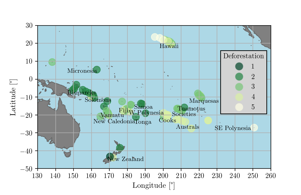
Deforestation is measured on a scale from 1 to 5, where 5 means complete deforestation (which was the case e. g. for Easter Island). After the initial selection of the predictors, described in this Jupyter notebook, I ended up with these variables:
- Absolute Latitude (proxy for average temperature)
- Area (area of island, km2, logarithmic scale)
- Isolation (km to nearest island >25% size of home island, logarithmic scale)
- Elevation (highest point, m, logarithmic scale)
- Rainfall (at sea level, mm/y, logarithmic scale)
- Tephra (volcanic ash fallout based on location with respect to Andesite line: scale: 1 (low) - 3 (high))
- Individual Ownership (cultural variable, yes/no)
Model building and evaluation
The dataset was small (80 island-samples), so I had to be careful about overfitting. I used a nested cross-validation to score the models. The outer cross-validation followed Leave-1-Out principle, i. e. the model was trained on all but one sample. This procedure was repeated 80 times for each island, producing a distribution of 80 prediction errors. The inner cross-validation was meant to determine the best hyper-parameters of the models and followed Leave-3-Out principle with randomized selection of 40 sample-sets of size 3. This inner cross-validation was repeated for every Leave-1-Out outer cross-validation, reducing the bias of the final scores.
I tested the following models: Decision Tree, Random Forest, Ridge and Huber linear regressions. Baseline model is prediction of median deforestation level of 3 for each island.
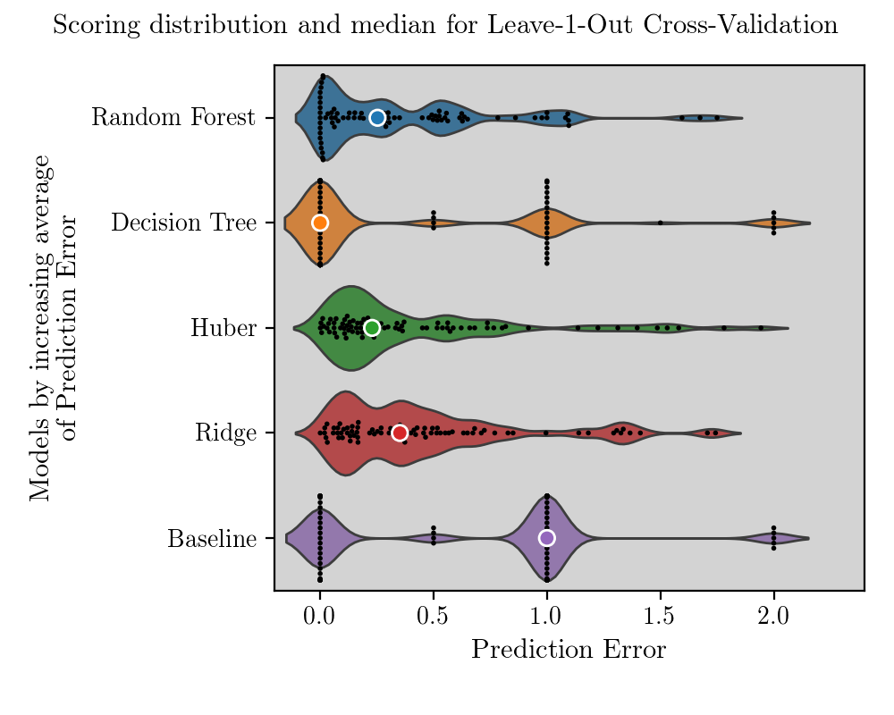
It is interesting to see that distributions of prediction errors are very different. Decision Tree predicts only discrete values of deforestation levels, since this is how they appear in the dataset. Random Forest and linear regressions have a moderately long-tailed distribution of prediction errors, but is is Random Forest which is superior since it has a great number of perfect predictions. Now we reduce the graph above and look at only two metrics of error distributions: average and median.
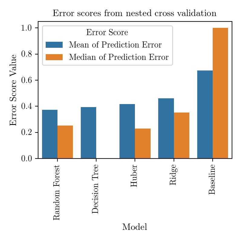
Now we can see that actually Huber linear regression performs on average almost as well as a more complex Random Forest. Especially when working with small datasets one should try to choose as simple model as possible, to reduce the overfitting resulting from variance within the dataset. However, a model like Random Forest could help uncover some non-linear interactions between the variables, which would be a step beyond standard linear regression analysis.
Importance of predictors
To establish the relative importance of predictors I used three proxys: normalized regression coefficients for linear regression models, tree feature importance provided by scikit-learn for tree models (which might not be a very reliable measure, read here), and permutation importance for all models. Note that results for Decison Tree are averegas over different realizations of trees, which depend strongly on the initial randomization (this is not the case for the other models).
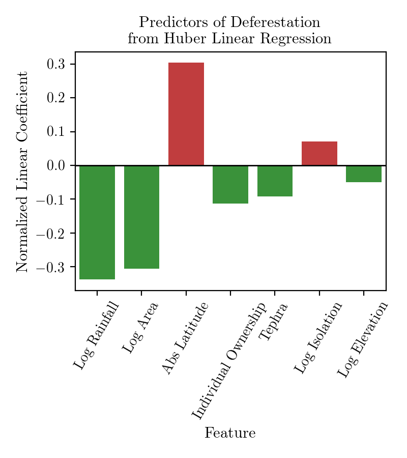
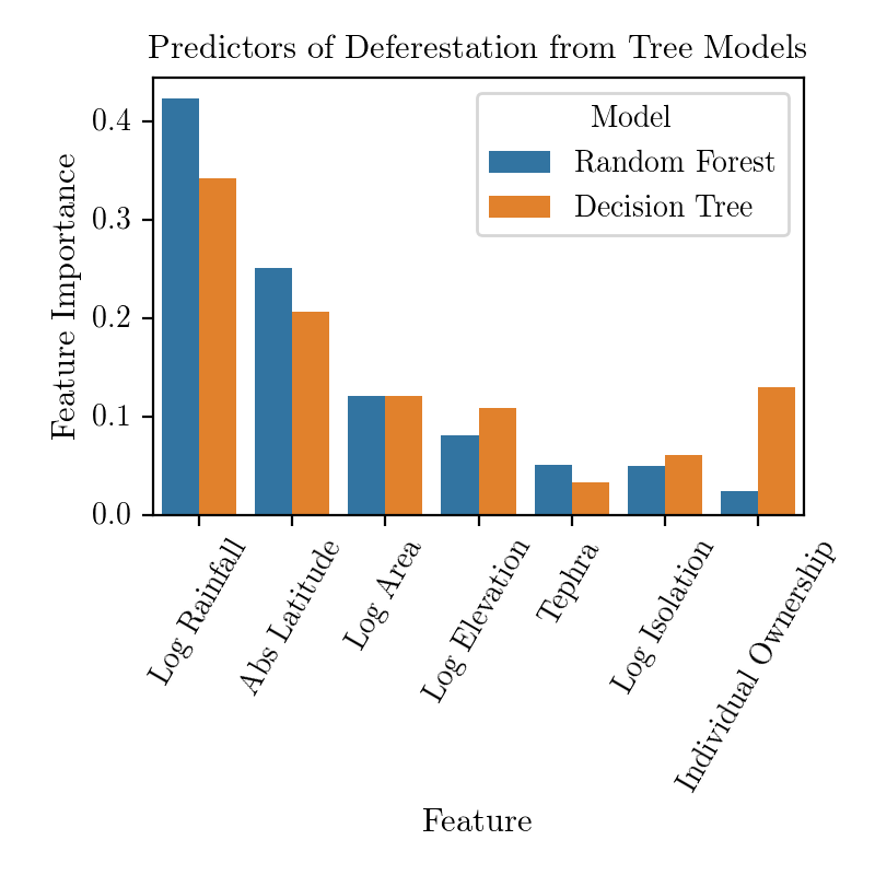
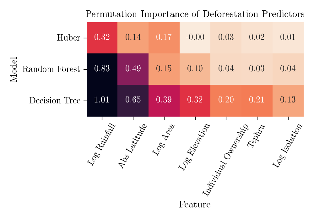
All the methods agree that Rainfall, Absolute Latitude and Area play the major role in determining the expected Deforestation. Let's now turn to an attempt to attribute the importance of individual variables to single predictions.
Explainability of predictions
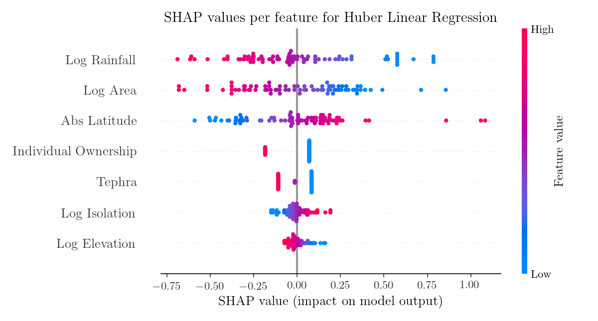
Recently, a method based on a game-theoretic Shapley value has been developed to "explain the output of any machine learning model" (SHapley Additive exPlanations, github.com/slundberg/shap). SHAP values have desirable properties as measures of feature contributions to a single outcome:
- they add up to the difference between the actual and average outcome,
- if the marginal contributions of two features are equal, so are their SHAP values,
- if a feature has no marginal contribution to the outcome (i. e. if it does not change the outcome), its SHAP value is 0.
For the two following plots I used models trained on the whole dataset.
In the case of linear models where the variables are assumed to be independent, SHAP values are monotonic functions of the variable values and don't bring much new insight.
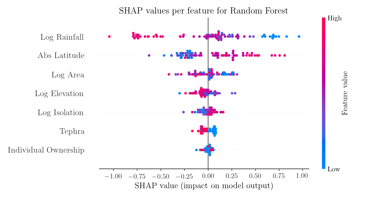
However, they can reveal interesting information when applied to general non-linear models, such as Random Forest.
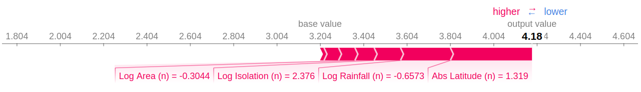
Eventually, I decided to see how well Huber regression and Random Forest predict high level od deforestation (5) on Easter Island and how SHAP values explain those predictions. This time the island for which the prediction is made is excluded from the training set. Huber linear regression predicts deforestation level 4.18.
The Random Forest model performs worse by predicting only 3.91.
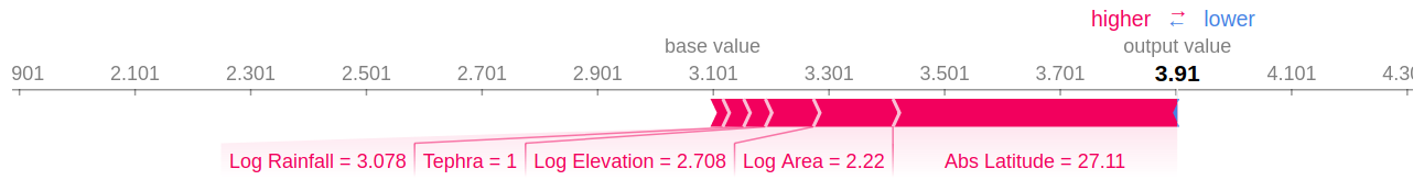
Both models agree that it is high latitude (low average temperature) that contributed the most to the deforestation. Actually, all the considered variables contributed positively to the deforestation outcome, pointing to the difficult environmental situation of the pre-European Easter Island society. However, the predicted deforestation is not as big as the one observed. At least two explanations are possible: the models do not describe the real trends well enough or there were some other variables, presumably cultural, that played an additional role.
Afterword
It was not the goal of this post to present a strict statistical analysis. A reader interested in more details of the actual research problem is encouraged to look at the original papers, whose results are not fully aligned with ours (and they differ between themselves too). The design of robust statistical analyses is in principle very hard, but I believe that machine learning can be of great help in this task.
The notebook with my analysis and the full repository with the dataset are linked below.
Comments
Comments powered by Disqus